tl;dr
- k-bisimulation can be used to create a condensed version of a graph. This condensed version is a graph summary, keeping specific properties of the original
- k-bisimulation partitions the nodes of the graph in equivalence classes which we call blocks
- We create the summary by creating one node for each block. Then, for each edge in the original graph, we connect the corresponding blocks with an edge, with the same label.
- To speed up the computation of the k-bisimulation, we
- use a partition refinement approach
- implemented everything in C++, making use of the boost libraries
- treat singleton blocks separately
- then treat blocks with only 2 nodes
- … and only then the rest
- devised a new step in the algorithm which remembers which parts might need to be refined from step k-1 to compute the blocks at step k
- Doing all this, we obtained a speedup of 20X compared to the already improved python implementation.
Introduction
When graphs get very large, they can become difficult to work with. One way to deal with such a graph is by reducing it to a smaller data structure which maintains the properties you want to preserve. In this specific case, we want to create a quotient graph based on a k-bisimulation. This summary graph preserves paths which were in the original graph, but can be much smaller than the original. For very large graphs, computing k-bisimulation is itself a challenge. There are existing frameworks, but they have their limitations. Some are either hard to set up and the overhead of the framework makes them less scalable. Often these frameworks trade efficiency for broader applicability; they have capabilities to produce a wider variety of summaries. In this blog post, we first define k-bisimulation and look at a naive algorithm to compute it. Then we will look into partition refinement, which is a faster way to compute the same thing. Finally, we will look at further optimizations of partition refinement and discuss how we implemented it.
k-bisimulation
We start from a labeled graph G = (V,E,L). where V is the set of vertices or nodes, L is a set of labels and E ⊂ {(v1,l,v2)|v1, v2 ∈ V and l ∈ L} is the set of labeled edges, also called the triples, of the graph. v1 is the source vertex of the edge, v2 is the target vertex. This definition implies that there can be multiple labeled edges between two vertices, but not two edges with the same label.
Now, we will start talking about paths in a graph. A path is a sequence of edges where the target vertex of the previous edge is the source vertex of the next edge. If we call the source of the first edge vstart and target of the last edge vend, then we say that this is a path from vstart to vend. The length of the path is the number of edges in the path. In some definitions it is assumed that an edge occurs only once in a path; we make no such assumption. Commonly, we are only interested in the labels of the edges in the path and not in the path itself. Therefore, we introduce the term labelpath to mean the sequence of labels of the path defined above. We define the set of all outgoing labelpaths of length k as pathsk, out(vA) to be the set of all labelpaths of at most length k starting at vertex vA (and ending anywhere in the graph).
Now we can find our k-bisimulation by first explaining when two vertices are bisimilar. Two vertices vA and vB are k-bisimilar if pathsk, out(vA) = pathsk, out(vB), i.e., they have the same set of labelpaths up to length k.
Side note: to be precise, we are working with forward-bisimilarity which deals with outgoing paths only. Analogously, backward-bisimulation deals with paths ending in a specific node. Forward-backward bisimulation deals with both at the same time, meaning that both incoming and outgoing paths must be equal.
What we now do to create the summary is first fixing the parameter k. Then, we use the bisimilarity as an equivalence relation between nodes, i.e., we consider two nodes equivalent if the are bisimilar. This equivalence relation identifies a partition on the vertices of the graph G, i.e., we can split the vertices E into subsets such that
- None of the subsets is empty and each vertex is in precisely one of the subsets.
- In each set, each vertex is bisimilar to all other vertices in that set.
- No vertex from one subset is bisimilar to a vertex from another subset.
We call each of these subsets a block of the partition.
Now we are ready to create our summary as follows. Given a graph G = (V,E,l) create a summary graph S = (VS,ES,l), where
- VS = {vB|B is a block in the partition}, i.e., we create one supernode for each of the blocks.
- ES = {(vA,l,vB)|(va,l,vb) ∈ E and A, B ∈ VS and va ∈ A and vb ∈ B}, i.e., for each edge in the original graph, we create a new edge, with the same label, between the vertices representing their blocks in the summary graph.
This kind of summary graph is a quotient graph.
To create these summaries the main algorithmic step is to compute the partition, i.e., find the subsets. After that, creating the edges is trivial.
A naive partition function.
A naive way to find the blocks is by computing all outgoing labelpaths for all nodes. This works as follows (python pseudo-code):
def find_paths (v: Vertex, k: int):
    labelpaths = set()
    for label, target in v.outgoing_edges():
        if k == 1:
            labelpaths.add([label])
        else:
            for deeperpath in find_paths(target, k - 1):
                labelpaths.add([label].extend(deeperpath))
    return paths


equivalence_map = defaultdict(list)
for v in V:
    paths = find_paths(v)
    equivalence_map[paths].append(v)
In this algorithm, for each vertex, we compute the set of all outgoing labelpaths. Then, we use the equivalence_map to make sure all vertices with the same set of paths get grouped together. In the end, the values in the map are the blocks we are looking for.
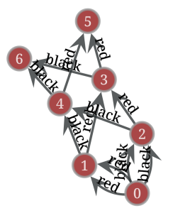
The problem with this implementation is that in the worst case the speed and memory use become quadratic in the depth of the path. This happens, for example, with graphs which look like the one in the figure.

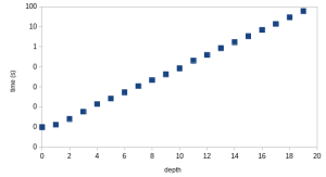
Here, the depth of the paths is only 3, which will not cause an issue. An issue arises when we encounter such structures with longer paths. If we make a larger graph with the same structure as the one above but with depth k instead of 3, we observe that the number of paths becomes 2k, which for a large k means very many paths. The following figure shows the outcome of an experiment for increasing depths.

What we see is that the time to execute becomes ever longer with an increasing depth (note the logarithmic scale on the y-axis). In general, we can see that this type of algorithm can behave exponentially. In effect, this implementation is not scalable for deep paths. Also when paths are shorter, this implementation is far from scalable for large graphs because of the large amount of data stored for the paths.
Towards a more efficient implementation
As usual in computer science, everything has been solved in the 80-ies. Also in this case. In the paper
@article{doi:10.1137/0216062,
    author = {Paige, Robert and Tarjan, Robert E.},
    title = {Three Partition Refinement Algorithms},
    journal = {SIAM Journal on Computing},
    volume = {16},
    number = {6},
    pages = {973-989},
    year = {1987},
    doi = {10.1137/0216062},
    URL = {https://doi.org/10.1137/0216062}
}
the partition refinement algorithm was used to compute bisimulations. The lingo used in the paper is rather different, but the algorithm almost directly applies. There are a few differences, though. In that work, the authors did not care about k, but were only interested in the case where k reaches infinity, meaning that all paths, independent on length must be the same for vertices to be bisimilar. We hence adapted the algorithm to our use case. Here, I explain the intuition behind the algorithm.
Partition refinement
As mentioned the algorithm is called partition refinement. It works by creating a partitioning for a depth k − 1, and then refining that partition to become the one for level k of the bisimulation. In other words, when we need to compute k-bisimulation, we assume (k-1)-bisimulation has already been computed. In other words, the algorithm works inductively.
For k = 0, meaning paths of length 0, all vertices are equivalent. So we define the partition to contain one block that contains all vertices.
For k > 0, we assume the (k−1)-bisimulation has been computed already. This one has a number of blocks. The vertices within each block are pairwise (k−1)-bisimilar.
Now, we work block by block through the blocks at level (k−1). For a given block A, we compute a signature for each of the vertices. For a vertex va, this signature consists of the set of all (l,B) for which (va,l,vb) ∈ E and vb ∈ block B on level (k−1).
Based on these signatures, we are splitting block B, into smaller blocks, where each new block contains the vertices which have the same signature. These blocks are added to the collection of blocks for level k. After this, we throw away the signatures and continue with the next block.
Correctness of partition refinement
It is important to realize that the partition refinement algorithm will result in precisely the same final partition as the original algorithm. You can either believe this, and skip this section, or follow the informal argument. If that does not convince you, you could read a more formal proof in the original paper, specifically section 3 ‘Relational coarsest partition’.
We need to show the three properties:
- None of the blocks is empty and each vertex is in precisely one of the blocks.
- In each block, each vertex is k-bisimilar to all other vertices in that block.
- No vertex from one block is k-bisimilar to a vertex from another block.
First, it is trivial that none of the blocks is empty, and that each vertex is in precisely one block because we encounter each vertex only once iterating over the blocks.
For the second property, let’s look at two vertices in a block at level k. The vertices which ended up here had the same signature. If we look at one element (l,B) of the signature, we realize that both vertices have one (or more) outgoing edges with label l which end up in a vertex in block B. But, by induction, the vertices in block B are (k−1)-bisimilar, meaning that all of them have the same sets of outgoing paths. Prepending all these paths with l still results in two sets with the same paths. So, each part of the signature results in a set of paths which are the same for both vertices. Hence, this pair of vertices, and by extension all pairs of vertices in the block are k-bisimilar. We chose an arbitrary block, so in all blocks on level k the property holds.
We can show the third property by contradiction. Imagine the property holds for the previous round and now we find two vertices va and vb which are k-bisimilar and in different blocks in the current round. To be k-bisimilar, these two vertices need to be (k−1)-bisimilar. So, in the previous round, they must have been in the same block B. And therefore, their signatures were directly compared. The only way they could have ended up in different blocks is if their signatures were not the same. This can have two causes.
- One of the labels might be different. This, however, means that the vertices are not k-bisimilar which is a contradiction.
- We find a part of the signature for va which has the same label, but ends in a block A, rather than the corresponding part in the signature for vb, which refers to block B. (if this is not the case, invert the roles of va and vb). However, we assumed all was fine until the previous round. This means that va has an edge to a vertex in block A, while vb does not have an edge to a vertex in block A. Since the vertices in block B are not (k−1)-bisimilar to the vertices in block A, va and vb are not k-bisimilar, which is a contradiction.
So, given that all three conditions are fulfilled, we are guaranteed a correct k-bisimulation with this algorithm.
Efficient implementation in Python
The theoretical result is interesting, but we apply a few additional insights to speed up the computation.
- When no refinement is happening, we know that we are done, and can stop. This happens at the latest when the number of rounds becomes equal to the diameter of the graph.
- When a block only contains one element, ie., it becomes a singleton, we never have to look at it again. It can also be stored more efficiently: instead of storing a list to contain all vertices in the block, we can have one list containing all vertices which are in a singleton block at this round. These can just be extended with new singletons in the next round.
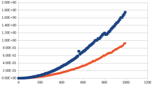
With these tricks applied, we reduced the runtime of the bisimulation algorithm significantly. The following figure shows the runtime on the same type of graphs which illustrated the exponential behavior above. Now, we see that running a graph with depth 20 takes under 0.10 seconds, rather than the 100 seconds needed before. Even using a depth of 1000 results in a runtime of less than 2 seconds.

Now, we were ready to run this algorithm on a large graph. We chose a DBpedia dump which contains 8 million entities, and about 22 million edges. And ran it on a laptop with a i7-1280P CPU. The bisimulation ran until it reached k=146 before it finished. It took about 12 minutes 39 seconds, including about 40 seconds to load the data. It used about 40GB RAM.
To scale this up further, we had some more ideas, some of which would need more control on the memory management. We therefore moved to implement this in C++.
Efficient implementation in C++
For the implementation in C++ we heavily relied on the Boost libraries which provide efficient unordered container types like flat sets and flat maps. We also made use of emplacement to avoid object copying when possible. Besides the optimizations done for the Python version, we further optimized the following:
- We keep track of which blocks have been split at the previous round. Only blocks which have vertices with edges to these blocks can be split at the next round. As far as we know, this is a novel addition to the algorithm.
- We also experimented with a reverse index which keeps track of these edges directly, this did however not lead to significant speedups
- We keep a mapping from the vertices to the block in which they are.
- We specialize this for level zero because everything is in the same block.
- We do not keep singletons explicitly. Rather, we map the corresponding vertices to negative integers, which indicates that they are singletons. To keep track of singletons blocks, we only need to remember how many there were.
- After the round, the index of the previous round is cleared as is is no longer needed.
- To create the blocks at level k, we first create a shallow copy of the blocks at level k-1. Only the modified block will occupy additional memory, others will only occupy one pointer.
- When splitting blocks, we try to not move all the data around. Rather, we put the first part of the split in place of the old block and put the other new parts in the back, then we update only the necessary mappings.
- In some cases, a split results in only singletons. In that case, we add a special empty block to the result. As soon as possible, that block will be overwritten by other splits, which will be put in these places, rather than appended to the back. Note that in a rare case an empty part could remain. This might contradict the requirements. A final cleanup step, which is not yet implemented, could take care of this.
- We deal with blocks of size 2 first, because when they split, they cause two singletons, and always an empty block. The heuristic is that by doing these first that there is a larger chance that larger blocks will not just split into singletons and fill this gap.
With these additional steps, we could further reduce the running time for the DBpedia dataset. This now runs in 56 seconds, including 20 seconds for reading, meaning 36 seconds for the actual computation. To compare, the python version needed 720 seconds (excluding reading). The speedup is about a factor 20. The memory usage went down from 40 GB to 10.7GB, so roughly by a factor 4.
Further details
Both implementations also have a support parameter, which defaults to 1. If the size of a block goes under that size, then the block will no longer be a candidate for splitting.
It would be possible to port some of the optimizations from the C++ version back to the python version.
Further possible optimizations
It would be possible to only partially compute the signatures until enough of it is computed to notice a difference where a node gets into a singleton block. This would, however, require quite some bookkeeping and that is most likely outweighing potential gains.
Michael Cochez – Assistant Professor, Vrije Universiteit Amsterdam

