
What is graph sampling?
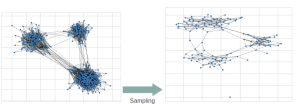
With the growing size of graphs in the real world, reducing their complexities becomes increasingly essential and computationally demanding, and due to the unavailability of whole graphs for privacy or scalability reasons, gathering relevant samples for analyzing and estimating their features is crucial. Therefore, several graph sampling algorithms emerged to simplify huge graphs.
Sampling Methods
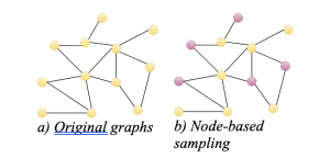
Graph sampling methods fall into three categories:
- Node-based
The simplest algorithms for sampling graphs involve selecting nodes and their connections. Different algorithms vary in how they choose nodes, whether it’s randomly or based on certain criteria to prioritize nodes with high degrees or PageRank scores. However, some of these methods may not fully capture the degree properties of the graph.
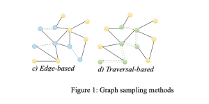
- Edge-based
Edge-based samplings are straightforward sampling methods that preserve edge-dependent properties, such as path length. However, they might mostly sample high-degree nodes and harm the graph structure.
- Traversal-based
Traversal-based methods enhance the performance of node and edge-based methods by taking into account the topological information of a graph. These methods involve exploring the graph’s structure, which can be categorized into random walk (RW) based methods and neighborhood exploration methods. The RW-based methods encompass various approaches such as random jump and Metropolis-hastings RW, which involve randomly traversing graph edges based on different policies. On the other hand, neighborhood exploration methods entail exploring the neighbors of a seed set based on specific criteria or objectives. Examples of this category include snowball, forest fire, and expansion sampling. While these approaches can preserve structural and degree information, they may be time-consuming depending on the graph’s structure. Moreover, they may yield local sampling if the seeds are not sufficiently spread out or if the walks become confined to a specific region.
Analyzing graph sampling methods: why?
In this blog, we evaluate various traits of samples produced by the different sampling methods.
Some methods are successful at preserving specific distributions like degree and clustering coefficient, as well as distances, while others are even more efficient. Additionally, the quality of these samplings and their outcomes can rely on graph properties, such as the number of nodes/edges, various centralities (e.g., betweenness and eigenvector), and nodes’ distances to describe their shape.
It is crucial to rely on high-quality sampling for accurate results.
Due to the presence of multiple sampling algorithms, it is important to anticipate their outcomes to avoid unnecessary sampling, which can consume time and memory.
How do we evaluate sampling? By the quality of samples.
We can use various quality metrics to assess sampling outcomes, depending on which aspect of the graph we want to prioritize. These can include the distributions of nodes’ degrees, clustering coefficient, and the distances between nodes (hop-plots). We then measure the divergence between the intended properties of the original and sample graphs using divergence metrics such as Kolmogorov-Smirnov and Jensen Shannon divergence.
Efficiency of sampling
As before mentioned, the need is often to sample from large graphs, which can be time-consuming. Therefore, an efficient algorithm is required to produce samples quickly.
How we predict sampling outcomes?
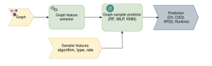
It’s essential to analyze the outcomes of sampling algorithms, whether through analytical or empirical research. The goal of Graph-Massivizer is to predict the quality of the sampling outcome or its execution time for a given sampling algorithm and input graph. To accomplish this, we start by extracting graph features to characterize it as an input to the prediction model.
Feature extraction and selection
Let’s now talk about the features that can help us predict outcomes in a graph. When it comes to graphs, we have different features to look at, like size and structural features. Size features tell us about the numbers of nodes and edges in the graph, while structural features describe the shape of the graph, including its diameter, node influence level, and betweenness centralities.
For size features, we have:
• Node/Edge numbers
And for structural features, we have:
• Density which shows the proportion of edge numbers among possible edges
• Clustering coefficient that tells us about the level of clustering around each node
• Shortest path length between nodes that gives us the minimum sequence length of edges connecting nodes
• Eigenvector/PageRank centrality showing the authority level of a node
• Betweenness centrality informing us about the level of nodes appearing in the shortest paths
• Degree assortativity that shows the level of similar degree nodes connected to each other
• Minimum spanning tree degree representing the degrees of the minimum tree covering all nodes
• Connected component sizes that gives us the sizes of connected regions
But the most important thing to remember is that not all these features may be relevant to what we’re trying to predict.
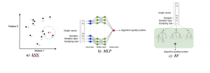
To avoid using unnecessary features, we use mutual information analysis to select the most relevant ones. This analysis helps us find non-linear connections between graph features and the outcome of the prediction model, which could be the desired quality metric or runtime. We also consider the sampling features, including the sampling algorithm, its type (node, edge, or traversal-based), and sampling rate for the model. When it comes to predicting the quality/runtime of sampling, we treat it as a regression problem. We use three machine learning models for this:
• random forest (RF),
• multilayer perceptron (MLP),
• k-nearest neighbor (kNN).
More specifically,
RF is the ideal model for high-dimensional and discrete data features, as it is both generalizable and robust. It is particularly suitable for graph data with numerous features.
Additionally, MLP is a flexible model that is well-suited for high-dimensional data.
On the other hand, kNN is an efficient model with minimal hyperparameters and demonstrates strong performance in the presence of similar data points.
Prediction results
Our project Graph-Massivizer has implemented prediction models that can provide predictions with errors below 20% regarding clustering coefficient and hop-plot metrics for most of considered sampling algorithms. However, their accuracy is dependent on the sampling algorithms. Therefore, we can select among the models for prediction on each algorithm. Overall, we find RF to be a suitable model for predicting clustering coefficient and hop-plots for most sampling algorithms.
As high-quality sampling methods can be time-consuming, we need to consider the runtime to compromise between runtime and the quality of the sample. We provide an algorithm ranking method using the prediction models for execution times to guide algorithm selection. We find kNN to be the best runtime prediction model.
Conclusion
Our study conclusively demonstrates that leveraging sufficient graph features and incorporating realistic graph features for training models can enable accurate prediction of sampling algorithm quality and facilitate ranking based on runtime, thus offering a method for algorithm selection that considers the trade-off between quality and efficiency. Efficient feature extraction methods are essential for developing a practical model.
Author: Seyedeh Haleh Seyed Dizaji, Postdoctoral Researcher at Universität Klagenfurt